
The Promise and Problems of Reasoning Models
Reasoning models are the next frontier of LLMs; they’ve provided the breakthrough needed to continue the relentless increase in evaluation benchmarks we’ve seen since the release of ChatGPT-3.5 . They’re revolutionary, they’re accessible, they’re agentic.
They’re also very, very, slow.
They tackle difficult problems by producing “thinking tokens”. A traditional LLM will immediately begin producing the answer as soon as it has processed the user’s input. A reasoning model will potentially produce thousands of thinking tokens, considering options and working through the solution before it sends a single token back to the user.
However, along with the release of DeepSeek-R1 came small, open source, distilled models like DeepSeek-R1-Distill-Qwen-7B. While fast by LLM standards, these models were still too slow for our uses. At Intercom over the past year we’ve poured a huge amount of engineering effort into bringing the median start of the response from Fin down to 7 seconds. These new smaller, faster, reasoning models were multiples too slow to be used as a component of an agent as fast as Fin is.
Our AI group machine learning scientists posed the engineers in the AI Infra team a question: But could they be that fast? Ideally 3ms per token fast? They could then churn out 2000 tokens to think through a difficult problem and still be useful components.
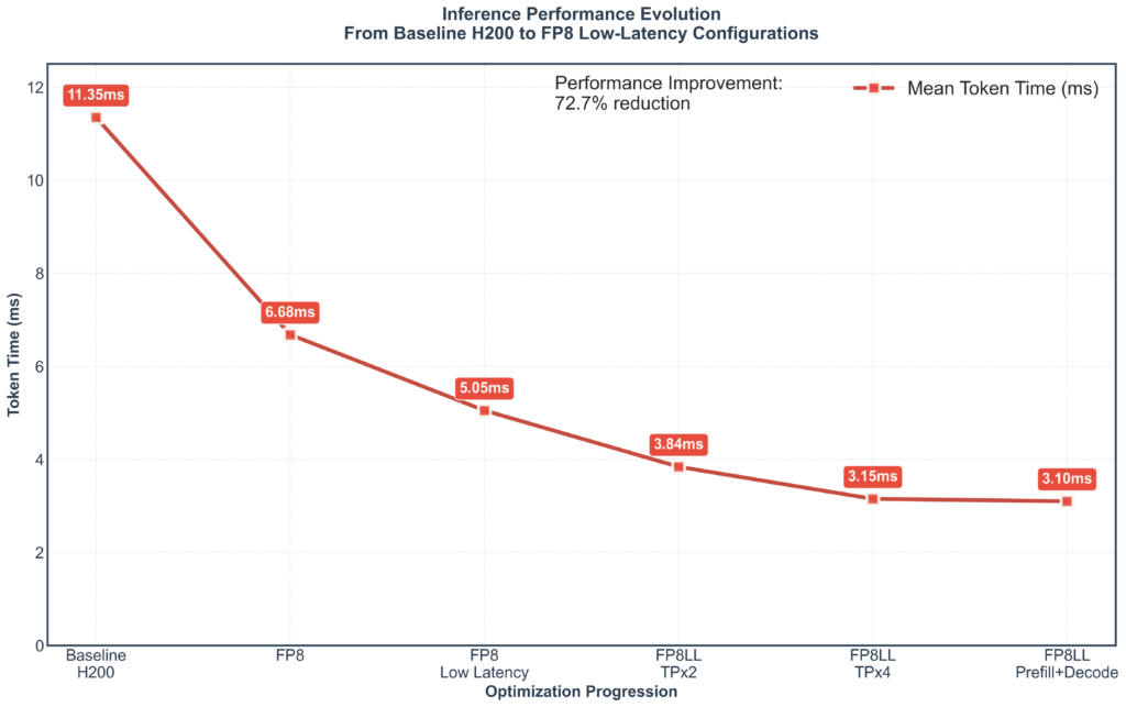
In this post we present the series of steps we took to reduce the inference time from 11.35ms down to 3.1ms. Most can be readily applied to any LLM and should be considered when putting a model into production. More interestingly we’ll present the rationale so that readers may know when to apply each optimisation themselves.
The optimisations applied were:
- Conservative quantization to FP8.
- Substituting low latency kernels.
- Tensor parallelisation to divide the work between GPUs.
- Prefill/decode disaggregated serving.
We’ll also discuss what didn’t work, and what we didn’t attempt and why.
Optimisation Process
Napkin math, Hardware and Software Choices
Before starting any optimisation process it’s useful to do some rough math to establish bounds and answer reasonable questions like “are we trying to break the speed of light today?”. Inference in LLMs is usually memory bandwidth bound due to the characteristics of modern GPUs. For instance, the Nvidia H200 can perform roughly 400 computations (floating point operations, or FLOPs) for each 16-bit parameter transferred — bandwidth is scarce relative to compute. Every single output token in a sequence requires us to load the entire model from memory and run the model’s calculations. A reasonable lower bound then on the physically possible is just “How long would it take to load the model from memory if we had no calculations, no overhead, and no coordination”. For DeepSeek-R1-Distill-Qwen-7B, a 7B model, at 16 bits/2 bytes per parameter then on a H200 with bandwidth of 4.8 TB/s this works out to:
$$T = \frac{14×10^9\:\textrm{bytes}}{4.8×10^{12}\:\textrm{bytes/s}}\approx0.002917\:\textrm{seconds}$$
Or about 2.9ms. So 3ms is possible! Or at least not ruled out by physical law.
It’s worth noting that this is an unusual optimisation task — usually the goal is to maximise throughput so as to minimise dollars per request. So another useful reference point is to see what result other similar efforts have had. Amazon’s inference hardware advertises a low latency approach of splitting a Llama 7B model across 24 cores for a final result of 7.7 ms. Others have found latency optimised deployments of 8B models could hit about 5ms on an H100 GPU. Significantly lower latency with larger models has been achieved using Nvidia’s newer Blackwell GPUs. Unfortunately, as of the time of writing, these GPUs are not widely available. Consequently, we’ll focus on the Hopper family of GPUs. The results obtained with Blackwell GPUs are further discussed in the Appendix.
What we’re really attempting to optimise here is the Inter-Token Latency or ITL. This is the average time between consecutive output tokens.
As mentioned, in concrete terms the ITL is the time it takes to load all the weights, do a single pass of the model’s calculations, and write the produced token back. We know GPUs are bandwidth-constrained, but just how much time should we focus on optimising the loading of the weights versus the speed of the calculations?
Thankfully, we already have the data for similar models. Taking a Llama 3.3 70B model running on an Nvidia H100 as an example: when processing a single sequence (no batching), it will spend ~100x as much time transferring the weights as doing the calculations.
The easiest optimisation we can make therefore is to just pick the GPU with the largest bandwidth. The H200 is widely available and has about 40% more bandwidth than the H100 for about 10% more cost, so that was ideal.
We chose the TensorRT-LLM inference engine as it provides a large number of optimisation options.
Benchmarking Approach
Many benchmarks found online focus on ChatGPT-like applications in ideal conditions where the number of input and output tokens are in the 100s. We were specifically undertaking this optimisation exercise to see if the model could operate fast enough for use within Fin. Fin is a production RAG system where prompts often contain thousands of tokens of relevant context and instruction.
Accordingly, we’ll begin using a representative set of 100 prompts drawn from one of the most challenging parts of Fin for an LLM. These prompts average 6000 input tokens, are only about 10% cacheable, and when answered by a non-reasoning model average 260 output tokens. The prompts are used as follows:
- A fixed Requests-per-second (RPS) is used to generate outputs for the entire sample to determine average time to first token (TTFT) and ITL. The number of tokens returned for a request is limited to the exact length of the expected response in the sample dataset to ensure apples-to-apples comparison between models despite output length variance.
- Repeated runs ramped the RPS up from 1 until the model’s performance passed a maximum TTFT and ITL.
This provides us with a good way to characterise the throughput and latency of the model in a way that allows quick iteration and easy comparison with other models we’ve benchmarked. The throughput figure should not be taken as a literal real-world expectation however due to differences in output length between reasoning and non-reasoning models and due to how LLM requests are load-balanced. It should be viewed as a proxy for the amount of load a particular configuration can serve, and how that configuration scales with increasing load.
Given this is not reflective of how a reasoning model would behave in production due to its much longer average output length, at the end of the iterative optimisation process we’ll show how to validate the low latency results under a benchmark that mimics real world reasoning model deployment with longer outputs.
Quantization
So, how can we further speed up transferring the bytes from memory? Cheat. Transfer fewer bytes. Quantization lets us reduce the amount of memory taken up by a model. Often used just to make large models fit into constrained GPUs’ memory it also crucially reduces the time taken to transfer the model to the compute units and calculate the next token. To minimise impact on the results of the model the conservative FP8 quantization method was chosen — essentially just 8 bit floating point numbers instead of the existing 16 bit (there’s more to it than that of course, scaling, calibration, test data, etc. — but this isn’t a blog on quantization). The Nvidia ModelOpt framework was used via TensorRT-LLM’s wrapper.
Even better, Hopper architecture Nvidia GPUs like the H200 contain specific hardware to accelerate FP8 calculations.
We evaluated the model post quantization using the MMLU and GSM8K benchmarks, the pre and post quantization results of the model are in the table below. This was the only step where we performed accuracy evaluation as all the other optimization steps we took are lossless — it’s the same operations with the same weights, just being performed in different orders, or in parallel.
| MMLU | GSM8K | |
| Base Model | 54.01 | 75.21 |
| FP8 Quantized Model | 54.03 | 71.53 |
| Change | -0.02 | 3.68 |
This step reduced ITL from 11.35ms to 6.68ms. A 40% reduction in latency to start with, or a 1.7x speedup. Not bad.
Low Latency Kernels
The advantage of TensorRT-LLM over alternate LLM inference servers like vLLM and SGLang is its level of configurability during its build phase. Instead of loading a HuggingFace model directly it first converts it to a standard intermediate format, during which it can quantize and perform other operations on the parameters. Then it converts the model into a TensorRT “engine” that can be loaded by Nvidia’s TensorRT optimised inference framework. At this point you can choose from a wide range of build options, two of which are low latency kernels for FP8 models, namely low_latency_gemm_plugin and low_latency_gemm_swiglu_plugin . By swapping in these kernels we get a further reduction in latency from 6.68ms to 5.05ms on a single H200. Another 24% relative reduction, a 1.3x speedup.
Tensor Parallelism
Tensor parallelism works by splitting large collections of weights across multiple GPUs. Operations that can be performed separately (such as large matrix multiplications) are then performed in parallel with the data being synced before operations that cannot be split. Tensor Parallelism in TensorRT-LLM is limited to a number of cards that divides evenly into the number of attention heads. Our model has 28 attention heads which results in a maximum tensor parallelism of 4 on an 8 GPU machine.
Splitting between 2 cards we see an improvement to 3.84ms and between 4 cards brings it down to 3.15ms. We see diminishing returns as tensor parallelism is less effective in situations like the one we were optimising:
- When your model or batch size is too small it becomes misaligned with the performance characteristics of modern GPUs which prefer to work on large matrices.
- When you’re not performing enough computation to mask the extra communication between the cards.
It may seem economically unwise to go from 2 to 4 GPUs, however it will provide headroom when we scale the throughput in the final optimisation step. Regardless, another 37% speedup or 1.6x faster. That’s >300 tokens per second, more than a page of a novel each second.
Disaggregated Serving and Throughput Scaling Result
LLM inference can be split into prefill phase (generating the first token by processing the entire prompt in a single forward pass, a slow and compute bound operation) and a decode phase (doing a much faster pass for every subsequent token produced) The length of the prefill phase determines the TTFT and the length of the decode phase determines ITL.
The prefill and decode phases can be separated onto different GPUs or even nodes. This is usually deployed due to its cost efficiency benefits:
- Different hardware can be used that more suits the compute or memory requirement of each phase.
- Even using the same hardware, if the limitation on throughput is that TTFT is too high you can use higher tensor parallelism in the prefill phase and if ITL is too high you can use more resources in the decode phase allowing you to decouple scaling requirements.
- The configuration of the inference engine can be completely tailored to the requirements of the phase — a larger number of tokens per forward pass for instance, something that benefits TTFT but slows ITL.
One less recognised advantage of disaggregated serving however is that it prevents the prefill phase from destroying the mean ITL of the decode phase.
Normally when a new request arrives while a previous request is still in the decode phase the server has two choices — pause the decode while doing the prefill of the new request, or batch them together using Continuous Batching (the vLLM term) or In-flight batching (the TensorRT-LLM term). This is illustrated in the diagram below.
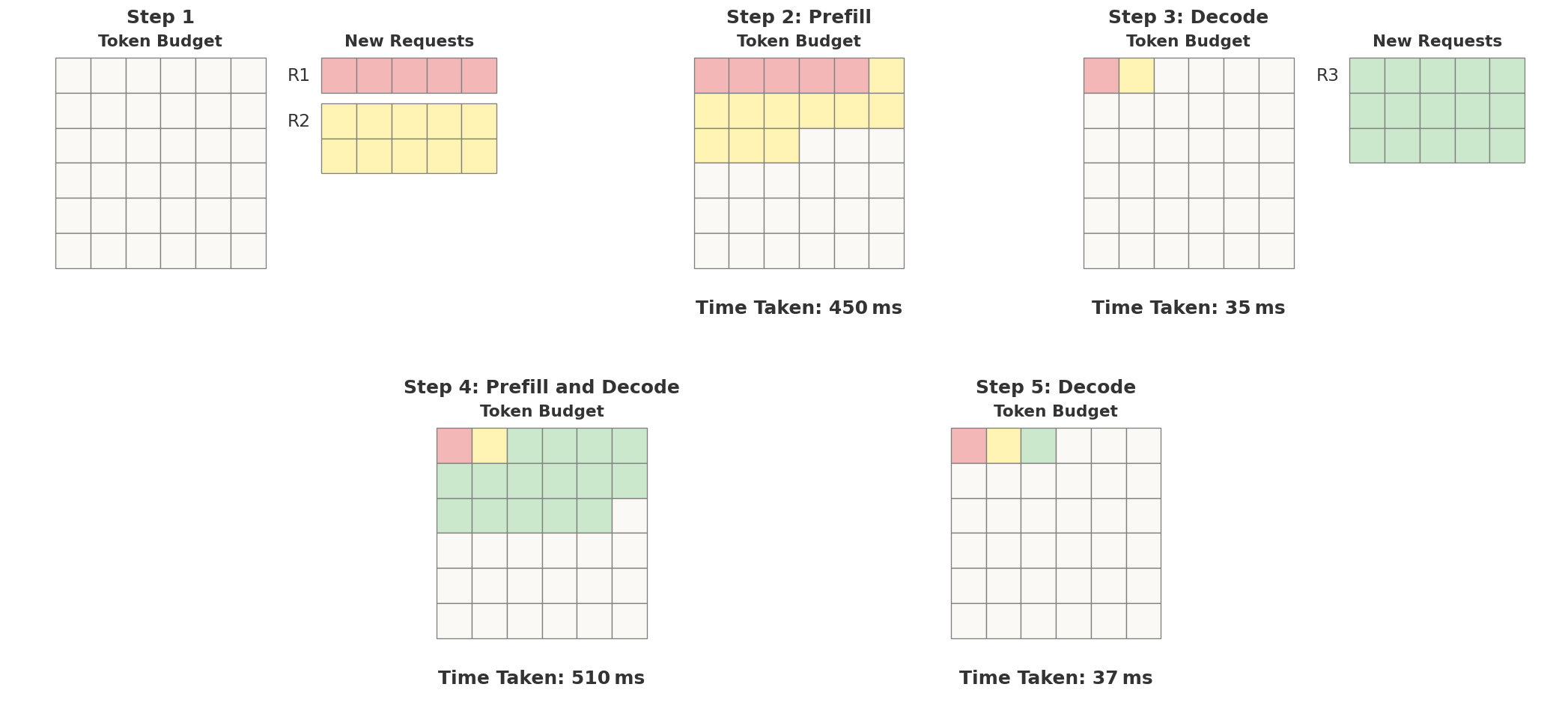
At step 1 two new prompts arrive in requests R1 and R2. At step two we allocate these to an inference step and do the entire prefill phase for R1 and R2, allowing us to now produce output tokens. At step 3 we do a decode phase for R1 and R2, producing the next output token for each sequence. During step 3 a new prompt arrives to begin R3. At Step 4 we do the decode for R1 and R2 but additionally do the prefill phase for R3. Finally at step 5 we do a decode for R1,R2, and R3.
We can see the problem immediately from the “time taken” figures in the diagram – mixing the prefill and decode phases results in wildly varying ITLs. If we separate out the prefill onto a different server we preserve ITL regardless of how many requests arrive.
In the case of our sample dataset the impact is even worse than is shown in the image as our prompts are 6000 tokens long.
Adding a server dedicated to the prefill phase reduces the latency from 3.15ms to 3.10ms. We leave the speedup calculation as an exercise for the reader. It might seem surprising given the above example but there’s a straightforward reason we’re seeing so little improvement — we’re sending 1 RPS. Each request is limited to producing ~260 tokens. The model is now so optimised that 260 tokens takes about 0.8 seconds, so overlaps between requests have become rarer.
Once we scale up the request rate however to determine the throughput limits of our architecture we see an entirely different story.
On the chart below you can see the throughput scaling of a server using only 4 way tensor parallelism vs adding a single prefill server. Adding a single prefill server increases the maximum throughput with acceptable latency from under 30k tok/s to over 50k tok/s.
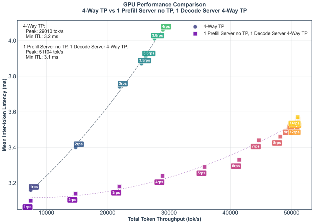
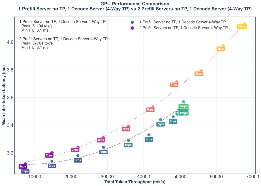
However we’re hitting a wall once the requests per second pass 8 or so. This is due to the single prefill server hitting its limit, if we add another prefill server we can continue to increase the throughput again to over 60k tok/s while remaining below 4ms ITL, at the penalty of a slight ITL increase.
Unfortunately while the final result looks performant it’s completely ignoring the key benefit of the model — reasoning.
Reasoning Model Benchmarking, How and Why Does it Scale, and Cost Calculation
The advantage of reasoning models is that they scale at inference time by producing many extra thinking tokens to increase the quality of their outputs. However, this is a completely different scenario from the one we normally benchmark. Our standard benchmark approach limits the output to the length produced by non-reasoning models, and as a result the average output length is ~260. This is far too small for a reasoning model.
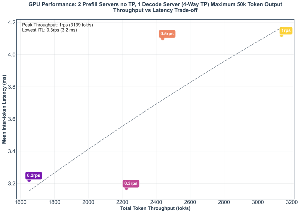
When we remove this output limitation this increases to ~1700 tokens on average — which at 3.1ms per output token would take 5.3 seconds to process, if we sent 7 RPS to a server it would quickly result in a very high rate of concurrency and thus latency.
The effect can be seen in the below chart where the 260 limit has been removed and tok/s craters to 3200 from over 60000 and RPS barely reaches 1 while exceeding 4ms ITL. This is exacerbated by the nature of reasoning requests where it is unpredictable how many thinking tokens each request will require resulting in much larger variance in concurrent requests.
So how would you actually serve this? Load balance intelligently. Inference Serving Frameworks like Nvidia Dynamo contain LLM aware routers that route requests away from already overloaded servers.
So to benchmark in a way that’s more relevant to the way a reasoning model would be deployed in production we switched from scaling RPS to find a realistic throughput to instead scaling the number of concurrent requests with unlimited output.
How Does it Scale, and Why?
The result is in the chart below. After 3 concurrent requests our performance exceeds our requirements.
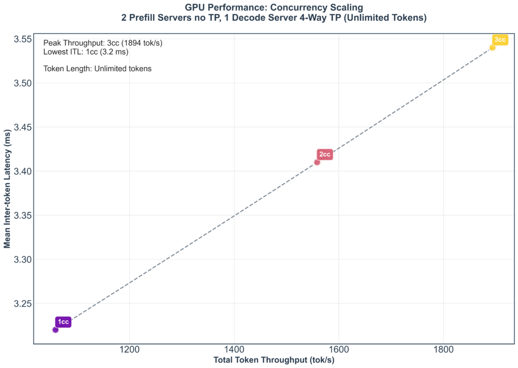
It may seem ridiculous that we top out at such a low number of concurrent requests — surely this isn’t the computational limit of the cards? The whole point of inference economics is that you can scale to large batches, serving many requests simultaneously for minimal extra performance penalty. Unfortunately that’s just not the problem we were optimising.
So, what’s the culprit? Memory yet again. We’ve reduced the model itself to about 7GB through quantization. If that’s the limiting factor on our speed then our performance will be sensitive to transferring relatively small amounts of data. Relatively small amounts like the KV cache.
The KV cache is an essential optimisation that turns the attention calculation at the core of the LLM from a quadratic operation to a linear operation per token. The tradeoff is that the size of the KV cache itself grows linearly with the length of the sequence being processed. In our case for a sequence of length 7500 it uses about 400MB. If you take the 3 concurrent requests into account this additional 17% use of memory bandwidth roughly matches the ITL increase we see as concurrent requests increase.
Still, it’s not all negative, an interesting aspect of this new scaling behaviour is that we’re only introducing a new request about once every 2 seconds. That’s >10x slower than we established a single prefill server can handle. As a result of us splitting the prefill and the decode we can move that computation to a much much cheaper machine. Or split the cost of a single prefill server using a H200 between many servers outputting tokens.
Costs and Conclusions
So, this must be prohibitively expensive? It depends. Let’s finish with some more napkin math.
The 4XH200 configuration we ended up with results in 3 requests every 6 seconds or so for our real world, long prompt use case — this is not a toy problem. That’s a request every 2 seconds. A standard AWS configuration for the H200 is 8XH200 in a single machine for ~$800 per day as of July 2025. We can host 2 decode servers on that single machine for a total output of 1 request completed per second, or 88400 per day. That works out at about a cent a request.
The appeal of reasoning models isn’t just that they solve problems better than prior LLMs, it’s that they also solve fundamentally different problems than LLMs, new problems.
So the question becomes, is solving these new, different, problems by making an open source reasoning model operate at application speeds worth 1c a request?
Appendix
Future Paths
More aggressive quantization
The FP8 quantization implemented is the most conservative quantization possible and while it was not optimised intensely it was chosen to maintain accuracy. Possible next steps that could be attempted include:
- Auto quantization down to 6 bits: TensorRT-LLM’s quantization framework allows autoquantization using a variety of quantization methods to bring the average number of bits used per parameter down further.
- AWQ and GPTQ quantization to test the effect on accuracy of reducing the model size down further to 4 bits.
- Manual choice of quantization on a per-layer basis can be performed.
Faster hardware — B200
The Blackwell B200 Nvidia cards have a memory bandwidth of 8TB/s or about 67% more than the H200 — this would be expected to provide a massive decrease in latency even without additional optimisations. Furthermore, just as the Hopper series introduced accelerated FP8 support, the Blackwell cards now offer FP4 support, expanding the options available for deploying low-latency, quantized models. Nvidia has demonstrated this capability on a system equipped with 8 B200 GPUs, achieving 1000 output tokens per second with the Llama 4 Maverick model and over 350 output tokens per second with the DeepSeek-R1 model (1k tokens in, 2k tokens out). These demonstrations involved extensive kernel-level optimisations, along with techniques discussed here, such as custom speculative decoding models and quantization.
Training Custom Speculative Decoding Models
Speculative decoding is the practice of producing multiple sequential candidate tokens on each forward pass that can then be evaluated on the next forward pass to potentially result in >1 tokens being accepted per iteration, and thus much lower latency. Approaches like EAGLE require a smaller compatible model to be trained that runs in tandem with the original model. While no pretrained model is provided for DeepSeek R1-Distill-Qwen-7B the paper does cover DeepSeek-R1-Distill-Llama-8B and reports a 5x speedup over baseline 16 bit decoding in ideal conditions. As reported later in the paper the results drop to a more modest 1.75x improvement for a Llama 8B model when tested in a production server setting (vLLM) with a batch size of 2, and benefits decrease as batch size increases.
Approaches that Failed or Weren’t Attempted
KV Cache Quantization
While the KV cache is a fundamental optimisation to modern LLM inference, it can take up a substantial amount of memory and thus occupy the memory bandwidth during inference. FP8 quantization of the KV cache was attempted, however the model appeared to be extremely sensitive to the optimisation as MMLU performance dropped to a score of 1.5 from a starting point of >50. Ideally an alternate quantization method would be more amenable to KV cache quantization with a potential total memory transfer reduction of ~8%.
Draft/Target Speculative decoding
Speculative decoding, as described above, is extremely promising for low latency inference. Unfortunately our use case has several aspects that reduced its likely benefit:
- Availability of appropriate draft models: The draft model produces candidate tokens that are evaluated on subsequent forward passes for their suitability by the main model. For the acceptance rate to be high enough to result in a latency decrease the model has to closely match the outputs of the main model. Unfortunately no suitably trained draft models existed — the mainline Qwen 2.5 0.5B model is incompatible with the 7B model for this purpose and community provided models were insufficient.
- Model size: For the greatest benefit there should be a large difference between the size of the main model and the size of the draft model. The size difference between a 7B model and a 0.5 model would likely result in much reduced speed improvement compared to often quoted results from 70B and >100B models. See squeezebits blog for details.
- Sequence length: Many of the tests used to benchmark speculative models have been benchmarks like GSM8K and HumanEval. GSM8K contains 40-80 tokens per question. The average prompt length for HumanEval is 67 words. Speculative decoding reduces in utility as sequence length increases, again see squeezebits blog for details.
Lookahead Speculative Decoding
Lookahead decoding is a form of speculative decoding that generates a pool of likely n-grams and then verifies them in a single forward pass similarly to other speculative decoding approaches. Ideally it results in single forward passes where n tokens are output for a possible n times reduction in ITL. TensorRT-LLM can apply this approach automatically and so it was straightforward to evaluate. Unfortunately though a range of parameters were tested the method appeared sensitive to the length of the prompt, with the fastest lookahead run being 33% slower than the unadjusted version.